In Chapter 2 of the textbook Practical Methods for Design and Analysis of Complex Surveys, Simple random sampling, systematic sampling and sampling with probability proportional to size are introduced as the basic sampling techniques. The estimation of three different population parameters (population total, ratio and median) is examined. A small fixed population – the Province’91 population - is used throughout to illustrate the estimation methods, where the main focus is on the derivation of appropriate sampling weights under each sampling technique. Special efforts are made in comparing the relative performances of the estimators (in terms of their standard errors) and the available information on the structure of the population is increasingly utilized. The use of such auxiliary information is considered for two purposes: the sampling design and the estimation of parameters for a given sampling design.

In Training Key 28, SRSWOR sampling is demonstrated by first reproducing the results of Example 2.1. Then, the SRSWOR estimation procedure is extended to samples with different sample sizes. Finally, the performance of SRSWOR estimators is examined by using Monte Carlo simulation methods.

In Training Key 45, intra-class correlation is demonstrated under systematic sampling. First, the results of Example 2.4 are reproduced. Then, intra-class correlation is examined for systematic sampling under varying sorting orders of the population.

In Training Key 54, PPS sampling is demonstrated by first reproducing the results of Example 2.6. Then, PPS sampling is examined in more detail by incorporating different types of auxiliary data into the estimation procedure.

2.2 The Province’91 population

Download SAS data | Download SPSS data | Download Excel file | Download text file

install.packages("tidyverse")
library(tidyverse)
province91 <- tribble(
  ~Stratum, ~Cluster, ~Id, ~Municipality, ~POP91, ~LAB91, ~UE91, ~HOU85, ~URB85,
  #-------|---------|----|--------------|-------|-------|------|-------|-------
  1, 1, 1, "Jyväskylä", 67200, 33786, 4123, 26881, 1,
  1, 2, 2, "Jämsä", 12907, 6016, 666, 4663, 1,
  1, 2, 3, "Jämsänkoski", 8118, 3818,   528, 3019, 1,
  1, 2, 4, "Keuruu", 12707, 5919,   760, 4896, 1,
  1, 3, 5, "Saarijärvi", 10774, 4930,   721, 3730, 1,
  1, 5, 6, "Suolahti", 6159, 3022, 457, 2389, 1,
  1, 3, 7, "Äänekoski", 11595, 5823, 767, 4264, 1,
  2, 5, 8, "Hankasalmi", 6080, 2594, 391, 2179, 0,
  2, 6, 9, "Joutsa", 4594, 2069, 194, 1823, 0,
  2, 7, 10, "Jyväskmlk", 29349, 13727, 1623, 9230, 0,
  2, 4, 11, "Kannonkoski", 1919, 821, 153, 726, 0,
  2, 4, 12, "Karstula", 5594, 2521, 341, 1868, 0,
  2, 8, 13, "Kinnula", 2324, 927, 129, 675, 0,
  2, 8, 14, "Kivijärvi", 1972, 819, 128, 634, 0,
  2, 3, 15, "Konginkangas", 1636, 675, 142, 556, 0,
  2, 5, 16, "Konnevesi", 3453, 1557, 201, 1215, 0,
  2, 1, 17, "Korpilahti", 5181, 2144, 239, 1793, 0,
  2, 2, 18, "Kuhmoinen", 3357, 1448, 187, 1463, 0,
  2, 4, 19, "Kyyjärvi", 1977, 831, 94, 672, 0,
  2, 5, 20, "Laukaa", 16042, 7218, 874, 4952, 0,
  2, 6, 21, "Leivonmäki", 1370, 573, 61, 545, 0,
  2, 6, 22, "Luhanka", 1153, 522, 54, 435, 0,
  2, 7, 23, "Multia", 2375, 1059, 119, 925, 0,
  2, 1, 24, "Muurame", 6830, 3024, 296, 1853, 0,
  2, 7, 25, "Petäjävesi", 3800, 1737, 262, 1352, 0,
  2, 8, 26, "Pihtipudas", 5654, 2543, 331, 1946, 0,
  2, 4, 27, "Pylkönmäki", 1266, 545, 98, 473, 0,
  2, 3, 28, "Sumiainen", 1426, 617, 79, 485, 0,
  2, 1, 29, "Säynätsalo", 3628, 1615, 166, 1226, 0,
  2, 6, 30, "Toivakka", 2499, 1084, 127, 834, 0,
  2, 7, 31, "Uurainen", 3004, 1330, 219, 932, 0,
  2, 8, 32, "Viitasaari", 8641, 4011, 568, 3119, 0
)
# save the population data for future use
save(province91, file="province91.RData")
# to download the population data use:
load(file="province91.RData")

Variables:

Stratum = Stratum identification 1=Urban, 2=Rural
Cluster = Cluster identification
Id = ID key
Municipality = Name of municipality
POP91 = Population in 1991 (Official statistics)
LAB = Labour force in 1991 (Official statistics)
UE91 = Unemployed in 1991 (Official statistics)
HOU85 = Households in 1985 (Population Census)
URB85 = Urbanicity in 1985 1= Urban, 0=Rural (Population Census)

THE PROVINCE91 POPULATION
Stratum	Cluster	Id	Municipality	POP91	LAB91	UE91	HOU85	URB85
1	1	1	Jyväskylä	67200	33786	4123	26881	1
1	2	2	Jämsä	12907	6016	666	4663	1
1	2	3	Jämsänkoski	8118	3818	528	3019	1
1	2	4	Keuruu	12707	5919	760	4896	1
1	3	5	Saarijärvi	10774	4930	721	3730	1
1	5	6	Suolahti	6159	3022	457	2389	1
1	3	7	Äänekoski	11595	5823	767	4264	1
2	5	8	Hankasalmi	6080	2594	391	2179	0
2	6	9	Joutsa	4594	2069	194	1823	0
2	7	10	Jyväskmlk	29349	13727	1623	9230	0
2	4	11	Kannonkoski	1919	821	153	726	0
2	4	12	Karstula	5594	2521	341	1868	0
2	8	13	Kinnula	2324	927	129	675	0
2	8	14	Kivijärvi	1972	819	128	634	0
2	3	15	Konginkangas	1636	675	142	556	0
2	5	16	Konnevesi	3453	1557	201	1215	0
2	1	17	Korpilahti	5181	2144	239	1793	0
2	2	18	Kuhmoinen	3357	1448	187	1463	0
2	4	19	Kyyjärvi	1977	831	94	672	0
2	5	20	Laukaa	16042	7218	874	4952	0
2	6	21	Leivonmäki	1370	573	61	545	0
2	6	22	Luhanka	1153	522	54	435	0
2	7	23	Multia	2375	1059	119	925	0
2	1	24	Muurame	6830	3024	296	1853	0
2	7	25	Petäjävesi	3800	1737	262	1352	0
2	8	26	Pihtipudas	5654	2543	331	1946	0
2	4	27	Pylkönmäki	1266	545	98	473	0
2	3	28	Sumiainen	1426	617	79	485	0
2	1	29	Säynätsalo	3628	1615	166	1226	0
2	6	30	Toivakka	2499	1084	127	834	0
2	7	31	Uurainen	3004	1330	219	932	0
2	8	32	Viitasaari	8641	4011	568	3119	0

Use dropdown in scatter plot below to toggle between variables.

TRAINING KEY 28: Analysing an SRS sample

INTRODUCTION

In this Training Key we use the Province’91 data set as a frame population in analysing an SRSWOR sample. In part A we calculate the SRSWOR estimates for the total of UE91 (number of unemployed in the province) and for the total of LAB91 (number of work force in the province) and their corresponding standard errors from the selected sample where sample size is eight \((n=8)\). In part B, we examine how sample size affects to the SRSWOR estimates and their standard errors by selecting different sample sizes. In part C we simulate SRSWOR samples by using Monte Carlo simulation techniques to examine the behaviour of the SRSWOR estimator. Part D is the option for interactive analysis.

A) ANALYSING AN SRS SAMPLE FROM THE PROVINCE’91 POPULATION

We calculate the SRSWOR (simple random sampling without replacement) total estimates of UE91 and LAB91, the ratio estimate (UE91/LAB91) and their corresponding standard error estimates. We use Province’91 data set as the frame population.

Start SAS Training Key

# Create a sample including Jyväskylä, Keuruu, Saarijärvi, Konginkangas, Kuhmoinen, Pihtipudas, Toivakka and Uurainen
Sample <- province91[c(1,4,5,15,18,26,30,31), ]
paste("SRSWOR sample is")

## [1] "SRSWOR sample is"

Sample

## # A tibble: 8 × 9
##   Stratum Cluster    Id Municipality POP91 LAB91  UE91 HOU85 URB85
##     <dbl>   <dbl> <dbl> <chr>        <dbl> <dbl> <dbl> <dbl> <dbl>
## 1       1       1     1 Jyväskylä    67200 33786  4123 26881     1
## 2       1       2     4 Keuruu       12707  5919   760  4896     1
## 3       1       3     5 Saarijärvi   10774  4930   721  3730     1
## 4       2       3    15 Konginkangas  1636   675   142   556     0
## 5       2       2    18 Kuhmoinen     3357  1448   187  1463     0
## 6       2       8    26 Pihtipudas    5654  2543   331  1946     0
## 7       2       6    30 Toivakka      2499  1084   127   834     0
## 8       2       7    31 Uurainen      3004  1330   219   932     0

#
# load package survey (to install package use: install.packages("survey"))
library(survey)
# total=32:  fpc = finite population correction: fpc = (1-n/N)
# This column (variable) fpc simply contains the number 32 for every record
Sample$fpc <- 32
# This variable contains the weights
Sample$weights <- 4
# Construct an object called province91.srs.design specifying a simple random sampling design. 
# This province91.srs.design object will be used for all subsequent analysis commands:
province91.srs.design <- svydesign(ids = ~1, data = Sample, fpc = ~fpc, weights = ~weights)
paste("Estimates for the total of UE91 and LAB91 under simple random sampling without replacement (SRSWOR)")

## [1] "Estimates for the total of UE91 and LAB91 under simple random sampling without replacement (SRSWOR)"

# Print the weighted total and standard error of the ue91 variable:
svytotal(~UE91, province91.srs.design)

##      total    SE
## UE91 26440 13282

# Print the weighted total and standard error of the ue91 variable:
svytotal(~LAB91, province91.srs.design)

##        total     SE
## LAB91 206860 109763

paste("Estimates for the ratio of UE91/LAB91 under simple random sampling without replacement (SRSWOR)")

## [1] "Estimates for the ratio of UE91/LAB91 under simple random sampling without replacement (SRSWOR)"

svyratio(~UE91, ~LAB91, province91.srs.design)

## Ratio estimator: svyratio.survey.design2(~UE91, ~LAB91, province91.srs.design)
## Ratios=
##          LAB91
## UE91 0.1278159
## SEs=
##            LAB91
## UE91 0.004087265

confint(svyratio(~UE91, ~LAB91, province91.srs.design))

##               2.5 %    97.5 %
## UE91/LAB91 0.119805 0.1358268

Selected SRSWOR sample and the estimates for the total of UE91 and LAB91 and for the ratio UE91/LAB91 are similar to the results viewed in table 2.4 on page 29 in Lehtonen and Pahkinen 2004. Pay attention to the estimates and their standard errors and try to think why SRSWOR may lack any significance for practical purposes according to this case study.

After viewing the results, you can examine the R and SAS codes used to calculate the estimates for the total of UE91 and LAB91 and for the ratio UE91/LAB91. Then, you may move on to next step of Key 28 in which different size SRSWOR samples will be selected to study how the sample size affects to the total estimate and to the ratio estimate.

B) SRS ESTIMATION WITH DIFFERENT SAMPLE SIZES

In this exercise we examine SRSWOR estimation of the total of UE91 (number of unemployed in the province) and LAB91 (size of labour force in the province) and of the ratio UE91/LAB91 by using different size SRSWOR samples. The purpose is to examine how sample size (\(n\)) affects to the total estimate and to the ratio estimate and their corresponding standard errors. We use Province’91 data set as the frame population.

Start SAS Training Key

Different sample sizes (n=4,8,16 or 32) of SRSWOR sample

Select the desired sample size from the tab below and view the results.

n=4

SRSWOR estimation for the total of UE91 and LAB91 and for the ratio UE91/LAB91 with different sample sizes

Province91 Population, Sample size = 4

# load packages
library(sampling)
library(survey)

# create function to select different size SRSWOR samples with user defined seed number
srs <- function(n, seed){
  print("Sample size is")
  print(n)
  set.seed(seed)
  # select a sample
  sampleprovince <- srswor(n,32)
  # the sample is
  (1:32)[sampleprovince==1]
  # selected data
  srs_sampledata <- getdata(province91, sampleprovince)
  print("Selected sample is")
  print(srs_sampledata)
  srs_sampledata$fpc <- 32
  srs_sampledata$weights <- (1/(n/32))
  # define design object
  province91.srs.design <- svydesign(ids = ~1, data = srs_sampledata, fpc = ~fpc, weights = ~weights)
  print("Estimate for the total of UE91 is")
  print(svytotal(~UE91, province91.srs.design))
  print("Estimate for the total of LAB91 is")
  print(svytotal(~LAB91, province91.srs.design))
  print("Estimate for the ratio of UE91/LAB91 and confidence interval is")
  print(svyratio(~UE91, ~LAB91, province91.srs.design))
  print(confint(svyratio(~UE91, ~LAB91, province91.srs.design)))
}
# Function srs(n, seed)
# Give sample size (n) and select your own seed number (seed). Call function srs().
srs(4,123)

## [1] "Sample size is"
## [1] 4
## [1] "Selected sample is"
##   ID_unit Stratum Cluster Id Municipality POP91 LAB91 UE91 HOU85 URB85
## 1      14       2       8 14    Kivijärvi  1972   819  128   634     0
## 2      15       2       3 15 Konginkangas  1636   675  142   556     0
## 3      19       2       4 19     Kyyjärvi  1977   831   94   672     0
## 4      31       2       7 31     Uurainen  3004  1330  219   932     0
## [1] "Estimate for the total of UE91 is"
##      total     SE
## UE91  4664 790.67
## [1] "Estimate for the total of LAB91 is"
##       total     SE
## LAB91 29240 4286.6
## [1] "Estimate for the ratio of UE91/LAB91 and confidence interval is"
## Ratio estimator: svyratio.survey.design2(~UE91, ~LAB91, province91.srs.design)
## Ratios=
##          LAB91
## UE91 0.1595075
## SEs=
##           LAB91
## UE91 0.01540906
##                2.5 %    97.5 %
## UE91/LAB91 0.1293063 0.1897087

n=8

SRSWOR estimation for the total of UE91 and LAB91 and for the ratio UE91/LAB91 with different sample sizes

Province91 Population, Sample size = 8

# load packages
library(sampling)
library(survey)

# create function to select different size SRSWOR samples with user defined seed number
srs <- function(n, seed){
  print("Sample size is")
  print(n)
  set.seed(seed)
  # select a sample
  sampleprovince <- srswor(n,32)
  # the sample is
  (1:32)[sampleprovince==1]
  # selected data
  srs_sampledata <- getdata(province91, sampleprovince)
  print("Selected sample is")
  print(srs_sampledata)
  srs_sampledata$fpc <- 32
  srs_sampledata$weights <- (1/(n/32))
  # define design object
  province91.srs.design <- svydesign(ids = ~1, data = srs_sampledata, fpc = ~fpc, weights = ~weights)
  print("Estimate for the total of UE91 is")
  print(svytotal(~UE91, province91.srs.design))
  print("Estimate for the total of LAB91 is")
  print(svytotal(~LAB91, province91.srs.design))
  print("Estimate for the ratio of UE91/LAB91 and confidence interval is")
  print(svyratio(~UE91, ~LAB91, province91.srs.design))
  print(confint(svyratio(~UE91, ~LAB91, province91.srs.design)))
}
# Function srs(n, seed)
# Give sample size (n) and select your own seed number (seed). Call function srs().
srs(8,123)

## [1] "Sample size is"
## [1] 8
## [1] "Selected sample is"
##   ID_unit Stratum Cluster Id Municipality POP91 LAB91 UE91 HOU85 URB85
## 1       3       1       2  3  Jämsänkoski  8118  3818  528  3019     1
## 2      10       2       7 10    Jyväskmlk 29349 13727 1623  9230     0
## 3      14       2       8 14    Kivijärvi  1972   819  128   634     0
## 4      15       2       3 15 Konginkangas  1636   675  142   556     0
## 5      18       2       2 18    Kuhmoinen  3357  1448  187  1463     0
## 6      19       2       4 19     Kyyjärvi  1977   831   94   672     0
## 7      22       2       6 22      Luhanka  1153   522   54   435     0
## 8      31       2       7 31     Uurainen  3004  1330  219   932     0
## [1] "Estimate for the total of UE91 is"
##      total     SE
## UE91 11900 5155.2
## [1] "Estimate for the total of LAB91 is"
##       total    SE
## LAB91 92680 44107
## [1] "Estimate for the ratio of UE91/LAB91 and confidence interval is"
## Ratio estimator: svyratio.survey.design2(~UE91, ~LAB91, province91.srs.design)
## Ratios=
##          LAB91
## UE91 0.1283988
## SEs=
##            LAB91
## UE91 0.006582346
##                2.5 % 97.5 %
## UE91/LAB91 0.1154976 0.1413

n=16

SRSWOR estimation for the total of UE91 and LAB91 and for the ratio UE91/LAB91 with different sample sizes

Province91 Population, Sample size = 16

# load packages
library(sampling)
library(survey)

# create function to select different size SRSWOR samples with user defined seed number
srs <- function(n, seed){
  print("Sample size is")
  print(n)
  set.seed(seed)
  # select a sample
  sampleprovince <- srswor(n,32)
  # the sample is
  (1:32)[sampleprovince==1]
  # selected data
  srs_sampledata <- getdata(province91, sampleprovince)
  print("Selected sample is")
  print(srs_sampledata)
  srs_sampledata$fpc <- 32
  srs_sampledata$weights <- (1/(n/32))
  # define design object
  province91.srs.design <- svydesign(ids = ~1, data = srs_sampledata, fpc = ~fpc, weights = ~weights)
  print("Estimate for the total of UE91 is")
  print(svytotal(~UE91, province91.srs.design))
  print("Estimate for the total of LAB91 is")
  print(svytotal(~LAB91, province91.srs.design))
  print("Estimate for the ratio of UE91/LAB91 and confidence interval is")
  print(svyratio(~UE91, ~LAB91, province91.srs.design))
  print(confint(svyratio(~UE91, ~LAB91, province91.srs.design)))
}
# Function srs(n, seed)
# Give sample size (n) and select your own seed number (seed). Call function srs().
srs(16,123)

## [1] "Sample size is"
## [1] 16
## [1] "Selected sample is"
##    ID_unit Stratum Cluster Id Municipality POP91 LAB91 UE91 HOU85 URB85
## 1        3       1       2  3  Jämsänkoski  8118  3818  528  3019     1
## 2        5       1       3  5   Saarijärvi 10774  4930  721  3730     1
## 3        9       2       6  9       Joutsa  4594  2069  194  1823     0
## 4       10       2       7 10    Jyväskmlk 29349 13727 1623  9230     0
## 5       11       2       4 11  Kannonkoski  1919   821  153   726     0
## 6       14       2       8 14    Kivijärvi  1972   819  128   634     0
## 7       15       2       3 15 Konginkangas  1636   675  142   556     0
## 8       18       2       2 18    Kuhmoinen  3357  1448  187  1463     0
## 9       19       2       4 19     Kyyjärvi  1977   831   94   672     0
## 10      20       2       5 20       Laukaa 16042  7218  874  4952     0
## 11      22       2       6 22      Luhanka  1153   522   54   435     0
## 12      23       2       7 23       Multia  2375  1059  119   925     0
## 13      28       2       3 28    Sumiainen  1426   617   79   485     0
## 14      29       2       1 29   Säynätsalo  3628  1615  166  1226     0
## 15      30       2       6 30     Toivakka  2499  1084  127   834     0
## 16      31       2       7 31     Uurainen  3004  1330  219   932     0
## [1] "Estimate for the total of UE91 is"
##      total     SE
## UE91 10816 2366.5
## [1] "Estimate for the total of LAB91 is"
##       total    SE
## LAB91 85166 19719
## [1] "Estimate for the ratio of UE91/LAB91 and confidence interval is"
## Ratio estimator: svyratio.survey.design2(~UE91, ~LAB91, province91.srs.design)
## Ratios=
##         LAB91
## UE91 0.126999
## SEs=
##            LAB91
## UE91 0.003543583
##                2.5 %    97.5 %
## UE91/LAB91 0.1200537 0.1339443

n=32

SRSWOR estimation for the total of UE91 and LAB91 and for the ratio UE91/LAB91 with different sample sizes

Province91 Population, Sample size = 16

# load packages
library(sampling)
library(survey)

# create function to select different size SRSWOR samples with user defined seed number
srs <- function(n, seed){
  print("Sample size is")
  print(n)
  set.seed(seed)
  # select a sample
  sampleprovince <- srswor(n,32)
  # the sample is
  (1:32)[sampleprovince==1]
  # selected data
  srs_sampledata <- getdata(province91, sampleprovince)
  print("Selected sample is")
  print(srs_sampledata)
  srs_sampledata$fpc <- 32
  srs_sampledata$weights <- (1/(n/32))
  # define design object
  province91.srs.design <- svydesign(ids = ~1, data = srs_sampledata, fpc = ~fpc, weights = ~weights)
  print("Estimate for the total of UE91 is")
  print(svytotal(~UE91, province91.srs.design))
  print("Estimate for the total of LAB91 is")
  print(svytotal(~LAB91, province91.srs.design))
  print("Estimate for the ratio of UE91/LAB91 and confidence interval is")
  print(svyratio(~UE91, ~LAB91, province91.srs.design))
  print(confint(svyratio(~UE91, ~LAB91, province91.srs.design)))
}
# Function srs(n, seed)
# Give sample size (n) and select your own seed number (seed). Call function srs().
srs(32,123)

## [1] "Sample size is"
## [1] 32
## [1] "Selected sample is"
##    ID_unit Stratum Cluster Id Municipality POP91 LAB91 UE91 HOU85 URB85
## 1        1       1       1  1    Jyväskylä 67200 33786 4123 26881     1
## 2        2       1       2  2        Jämsä 12907  6016  666  4663     1
## 3        3       1       2  3  Jämsänkoski  8118  3818  528  3019     1
## 4        4       1       2  4       Keuruu 12707  5919  760  4896     1
## 5        5       1       3  5   Saarijärvi 10774  4930  721  3730     1
## 6        6       1       5  6     Suolahti  6159  3022  457  2389     1
## 7        7       1       3  7    Äänekoski 11595  5823  767  4264     1
## 8        8       2       5  8   Hankasalmi  6080  2594  391  2179     0
## 9        9       2       6  9       Joutsa  4594  2069  194  1823     0
## 10      10       2       7 10    Jyväskmlk 29349 13727 1623  9230     0
## 11      11       2       4 11  Kannonkoski  1919   821  153   726     0
## 12      12       2       4 12     Karstula  5594  2521  341  1868     0
## 13      13       2       8 13      Kinnula  2324   927  129   675     0
## 14      14       2       8 14    Kivijärvi  1972   819  128   634     0
## 15      15       2       3 15 Konginkangas  1636   675  142   556     0
## 16      16       2       5 16    Konnevesi  3453  1557  201  1215     0
## 17      17       2       1 17   Korpilahti  5181  2144  239  1793     0
## 18      18       2       2 18    Kuhmoinen  3357  1448  187  1463     0
## 19      19       2       4 19     Kyyjärvi  1977   831   94   672     0
## 20      20       2       5 20       Laukaa 16042  7218  874  4952     0
## 21      21       2       6 21   Leivonmäki  1370   573   61   545     0
## 22      22       2       6 22      Luhanka  1153   522   54   435     0
## 23      23       2       7 23       Multia  2375  1059  119   925     0
## 24      24       2       1 24      Muurame  6830  3024  296  1853     0
## 25      25       2       7 25   Petäjävesi  3800  1737  262  1352     0
## 26      26       2       8 26   Pihtipudas  5654  2543  331  1946     0
## 27      27       2       4 27   Pylkönmäki  1266   545   98   473     0
## 28      28       2       3 28    Sumiainen  1426   617   79   485     0
## 29      29       2       1 29   Säynätsalo  3628  1615  166  1226     0
## 30      30       2       6 30     Toivakka  2499  1084  127   834     0
## 31      31       2       7 31     Uurainen  3004  1330  219   932     0
## 32      32       2       8 32   Viitasaari  8641  4011  568  3119     0
## [1] "Estimate for the total of UE91 is"
##      total SE
## UE91 15098  0
## [1] "Estimate for the total of LAB91 is"
##        total SE
## LAB91 119325  0
## [1] "Estimate for the ratio of UE91/LAB91 and confidence interval is"
## Ratio estimator: svyratio.survey.design2(~UE91, ~LAB91, province91.srs.design)
## Ratios=
##          LAB91
## UE91 0.1265284
## SEs=
##      LAB91
## UE91     0
##                2.5 %    97.5 %
## UE91/LAB91 0.1265284 0.1265284

C) SIMULATING SRSWOR SAMPLES BY USING MONTE CARLO SIMULATION TECHNIQUES

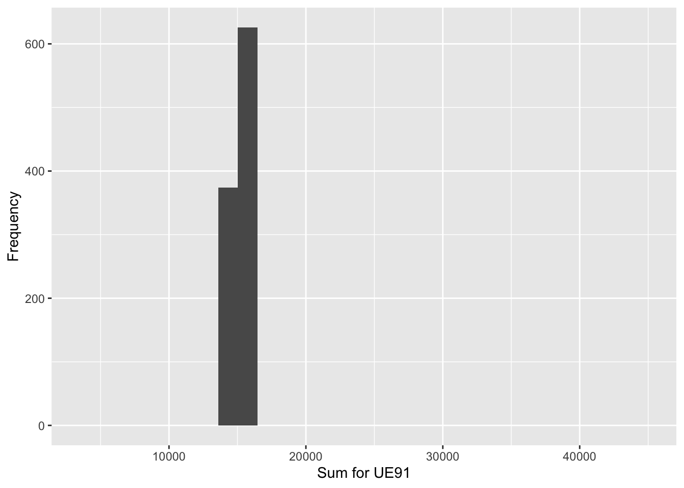
Monte Carlo simulations are performed to examine the behavior of the SRSWOR estimator.

Start SAS Training Key

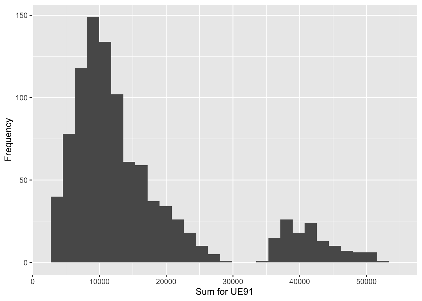
Simulation Experiments for SRSWOR estimator for the total of UE91

Select the desired sample size from the tab below and view the simulation results.

n=4

Sample size 4, Simulations 1000

**Simulation Experiments for SRSWOR estimator for the total of UE91.**
Population_Total	Mean_of_Estimates	Std	Bias
15098	15448.77	11228.39	350.768

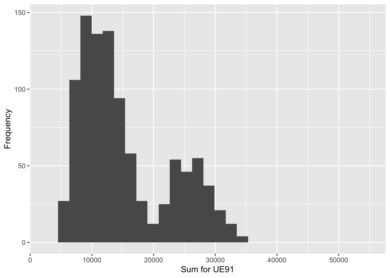
n=8

Sample size 8, Simulations 1000

**Simulation Experiments for SRSWOR estimator for the total of UE91.**
Population_Total	Mean_of_Estimates	Std	Bias
15098	15232.58	7281.658	134.58

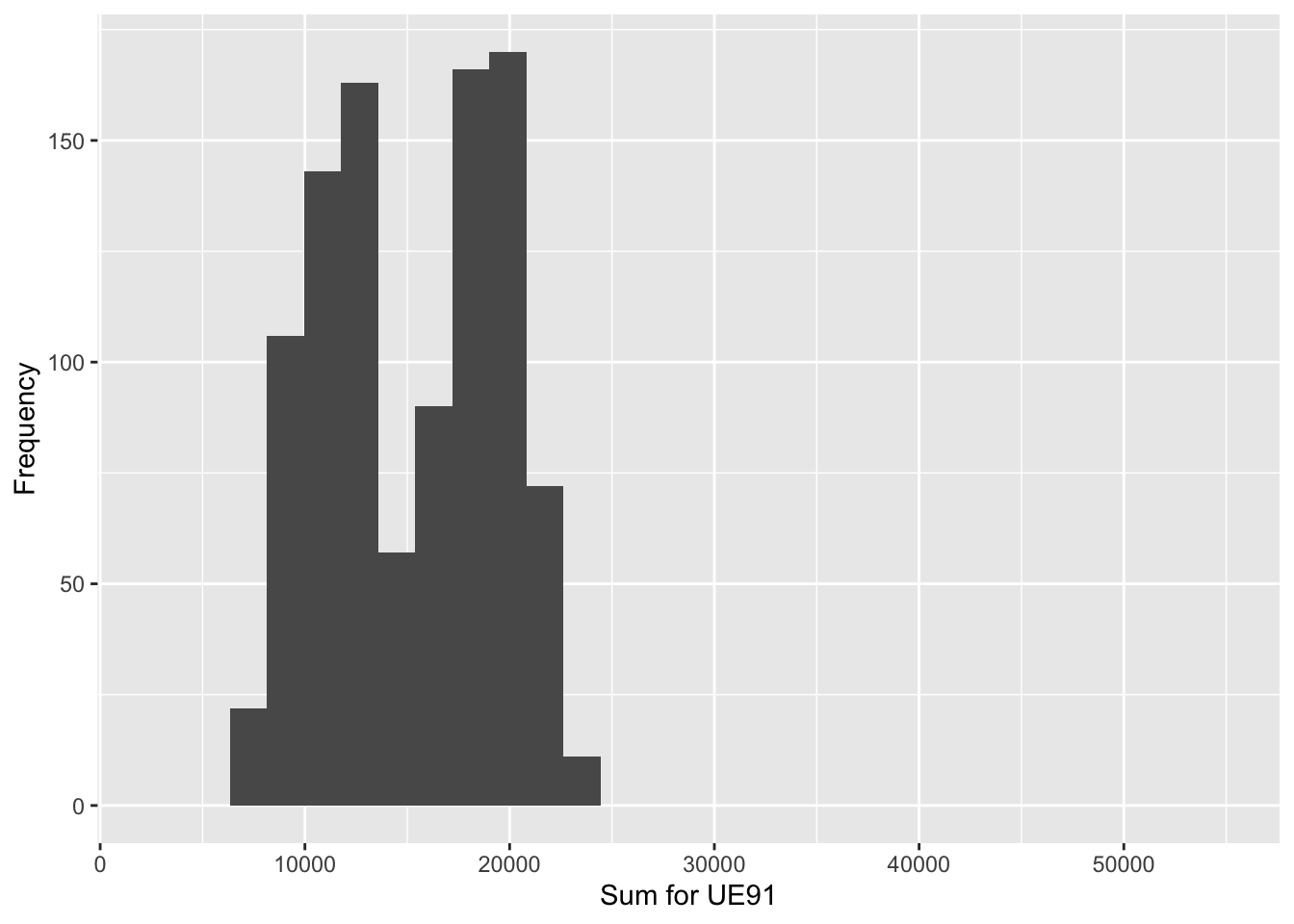
n=16

Sample size 16, Simulations 1000

**Simulation Experiments for SRSWOR estimator for the total of UE91.**
Population_Total	Mean_of_Estimates	Std	Bias
15098	15252.28	4265.515	154.276

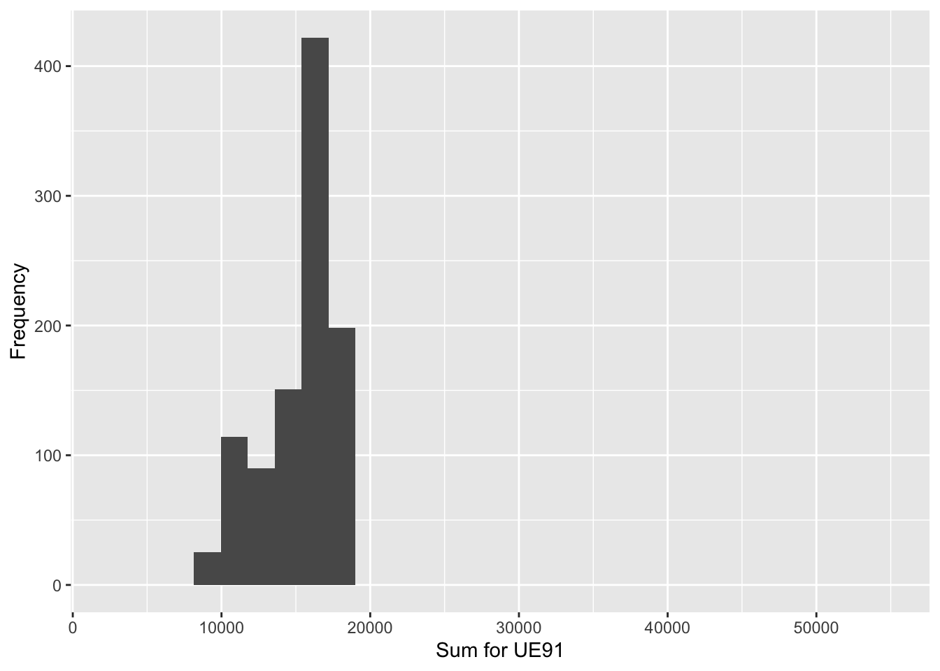
n=24

Sample size 24, Simulations 1000

**Simulation Experiments for SRSWOR estimator for the total of UE91.**
Population_Total	Mean_of_Estimates	Std	Bias
15098	15247.58	2368.397	149.584

TRAINING KEY 45: Intra-class correlation for systematic sampling

INTRODUCTION

In this Training Key we use the Province’91 data set as the frame population in calculating the intra-class correlation coefficient under systematic sampling. The total of the study variable UE91 (number of unemployed in the province) is to be estimated. In Part A, the book example will be worked out. The effect of different sorting orders of the population on the intra-class correlation will be examined in Part B. Part C provides an option for interactive analysis.

A) INTRA-CLASS CORRELATION FOR SYSTEMATIC SAMPLING IN THE PROVINCE’91 POPULATION

We calculate the intra-class correlation coefficient for systematic sampling involving four separate systematic samples of eight elements (see book example 2.4 on page 45). Further instructions will be given once you start.

Start SAS Training Key, NOT COMPLETED: a html file is missing

For the Province’91 population, four separate systematic samples of eight elements \((q=N/n=32/8=4)\) are drawn from the population data set. The total of the study variable UE91 (number of unemployed in the province) is to be estimated.

In systematic sampling, a certain design parameter exists. This parameter, called the intra-class correlation coefficient \(\rho_{int}\), will be included in the design variance \(V_{sys}\) of an estimator of the population total. The magnitude of the intra-class correlation, and consequently its effect on variance estimates, depends partly on whether there is a successive system of ordering of the study variable values in the population frame. The effect of sorting order is examined in Part B of this training key.

To calculate the intra-class correlation, the population variance is decomposed into the variation between the systematic samples and the variation within the systematic samples, as in standard one-way analysis of variance. In ANOVA terms we have \(SST = SSW + SSB\), where \(SST\) represents the total sum of squares, \(SSW\) the within sum of squares and \(SSB\) the between sum of squares. By using the decomposition of the total sum of squares, the intra-class correlation is defined as \(\rho_{int} = 1 - \frac{n}{(n-1)} \times \frac{SSW}{SST}\).

Systematic sampling compared with simple random sampling without replacement is

more efficient, if \(\frac{-1}{(n-1)} < \rho_{int} < 0\),
equally efficient, if \(\rho_{int} = 0\) or
less efficient, if \(0 < \rho_{int} < 1\).

In this exercise the intra-class correlation is negative (-0.08) which means that given the current sorting order of the population, systematic sampling will be more efficient than simple random sampling without replacement (SRSWOR). Note that the population was pre-sorted first by the variable URB85 (urbanicity) and within each URB85 class, by the variable Municipality for this exercise.

paste("Load frame Population data set Province'91:")

## [1] "Load frame Population data set Province'91:"

load("province91.Rdata")

Create four systematic samples: sample1, …, sample4.

sample1 <- province91[c(1,5,9,13,17,21,25,29), ]
paste("sample1 from population Province'91:"); sample1

## [1] "sample1 from population Province'91:"

## # A tibble: 8 × 9
##   Stratum Cluster    Id Municipality POP91 LAB91  UE91 HOU85 URB85
##     <dbl>   <dbl> <dbl> <chr>        <dbl> <dbl> <dbl> <dbl> <dbl>
## 1       1       1     1 Jyväskylä    67200 33786  4123 26881     1
## 2       1       3     5 Saarijärvi   10774  4930   721  3730     1
## 3       2       6     9 Joutsa        4594  2069   194  1823     0
## 4       2       8    13 Kinnula       2324   927   129   675     0
## 5       2       1    17 Korpilahti    5181  2144   239  1793     0
## 6       2       6    21 Leivonmäki    1370   573    61   545     0
## 7       2       7    25 Petäjävesi    3800  1737   262  1352     0
## 8       2       1    29 Säynätsalo    3628  1615   166  1226     0

sample2 <- province91[c(2,6,10,14,18,22,26,30), ]
paste("sample2 from population Province'91:"); sample2

## [1] "sample2 from population Province'91:"

## # A tibble: 8 × 9
##   Stratum Cluster    Id Municipality POP91 LAB91  UE91 HOU85 URB85
##     <dbl>   <dbl> <dbl> <chr>        <dbl> <dbl> <dbl> <dbl> <dbl>
## 1       1       2     2 Jämsä        12907  6016   666  4663     1
## 2       1       5     6 Suolahti      6159  3022   457  2389     1
## 3       2       7    10 Jyväskmlk    29349 13727  1623  9230     0
## 4       2       8    14 Kivijärvi     1972   819   128   634     0
## 5       2       2    18 Kuhmoinen     3357  1448   187  1463     0
## 6       2       6    22 Luhanka       1153   522    54   435     0
## 7       2       8    26 Pihtipudas    5654  2543   331  1946     0
## 8       2       6    30 Toivakka      2499  1084   127   834     0

sample3 <- province91[c(3,7,11,15,19,23,27,31), ]
paste("sample3 from population Province'91:"); sample3

## [1] "sample3 from population Province'91:"

## # A tibble: 8 × 9
##   Stratum Cluster    Id Municipality POP91 LAB91  UE91 HOU85 URB85
##     <dbl>   <dbl> <dbl> <chr>        <dbl> <dbl> <dbl> <dbl> <dbl>
## 1       1       2     3 Jämsänkoski   8118  3818   528  3019     1
## 2       1       3     7 Äänekoski    11595  5823   767  4264     1
## 3       2       4    11 Kannonkoski   1919   821   153   726     0
## 4       2       3    15 Konginkangas  1636   675   142   556     0
## 5       2       4    19 Kyyjärvi      1977   831    94   672     0
## 6       2       7    23 Multia        2375  1059   119   925     0
## 7       2       4    27 Pylkönmäki    1266   545    98   473     0
## 8       2       7    31 Uurainen      3004  1330   219   932     0

sample4 <- province91[c(4,8,12,16,20,24,28,32), ]
paste("sample4 from population Province'91:"); sample4

## [1] "sample4 from population Province'91:"

## # A tibble: 8 × 9
##   Stratum Cluster    Id Municipality POP91 LAB91  UE91 HOU85 URB85
##     <dbl>   <dbl> <dbl> <chr>        <dbl> <dbl> <dbl> <dbl> <dbl>
## 1       1       2     4 Keuruu       12707  5919   760  4896     1
## 2       2       5     8 Hankasalmi    6080  2594   391  2179     0
## 3       2       4    12 Karstula      5594  2521   341  1868     0
## 4       2       5    16 Konnevesi     3453  1557   201  1215     0
## 5       2       5    20 Laukaa       16042  7218   874  4952     0
## 6       2       1    24 Muurame       6830  3024   296  1853     0
## 7       2       3    28 Sumiainen     1426   617    79   485     0
## 8       2       8    32 Viitasaari    8641  4011   568  3119     0

# add sample IDs
sample1$sampleID <- 1
sample2$sampleID <- 2
sample3$sampleID <- 3
sample4$sampleID <- 4

# combine data sets
s <- rbind(sample1, sample2, sample3, sample4)

library(samplesize4surveys)
icc <- ICC(y = s$UE91, cl = s$sampleID)
paste("Intra-class correlation is"); icc$ICC

## [1] "Intra-class correlation is"

## [1] -0.08161488

The design effect is calculated by equation (2.24): \(DEFF_{sys}(\hat{t}) = \frac{V_{sys}(\hat{t})}{V_{srs}(\hat{t})} = 1 + (n-1) \times \rho_{int}\).

# Design effect
n <- nrow(sample1)
DEFF <- 1 + (n-1)*icc$ICC
paste("Design effect is"); DEFF

## [1] "Design effect is"

## [1] 0.4286958

In this exercise the design effect is DEFF=0.43 which implies that systematic sampling is very efficient in this case.

Further, we can write the design variance of the total estimator in the form

\(V_{sys}(\hat{t}) = N^2 \times (1 - \frac{n}{N}) \times \frac{S^2}{n} \times [1 + (n-1)\rho_{int}]\)

or alternatively

\(V_{sys}(\hat{t}) = V_{srs}(\hat{t}) \times [1 + (n-1)\rho_{int}]\), as is given in equation (2.23).

This also implies that systematic sampling is more efficient than SRSWOR when rhoint is negative.

B) INTRA-CLASS CORRELATION FOR SYSTEMATIC SAMPLING WHEN VARYING THE SORTING ORDER

We examine the effect of the sorting order of the Province’91 population on intra-class correlation. It will be shown that the sorting order matters: the value of the intra-class correlation coefficient varies much depending on the sorting order. Further instructions will be given once you start.

Start SAS Training Key

For the Province’91 population, four separate systematic samples of eight elements \((q=N/n=32/8=4)\) are drawn from the population data set similarly as in Part A. The total of the study variable UE91 (number of unemployed in the province) is to be estimated.

We now examine the effect of the sorting order of the population elements on the intra-class correlation coefficient. In sorting, we use the available auxiliary information on the population. The following sorting orders are developed:

Sorting by the variable URB85 (urbanicity in 1985), used in Part A
Sorting by the variable HOU85 (the number of households in 1985)
Sorting by the variable HOU85 (the number of households in 1985) and permuting
Sorting in random order by using a sequence of generated random numbers.

Sorting the population by one or several auxiliary variables before a systematic sample is drawn is sometimes called “implicit stratification” and is frequently used in practical application of systematic sampling.

E.g. results and code for sorting order d) (Sorting in random order by using a sequence of generated random numbers) is following. Try to change the sort variable (see code chunk below).

load("province91.Rdata")

# add random number for sorting
set.seed(123) # Pick a personal seed number
Random <- runif(nrow(province91), min = 0, max = 1)
province91 <- cbind(province91, Random)

# select variable for sorting (e.g. variable Random) and sort data 
province91.sorted <- province91[order(province91$Random),]
# try sorting by URB85 and HOU85 variables:
# province91.sorted <- province91[order(province91$URB85),]
# province91.sorted <- province91[order(province91$HOU85),]

# Create four systematic samples from sorted data 
sample1 <- province91.sorted[c(1,5,9,13,17,21,25,29), ]
sample2 <- province91.sorted[c(2,6,10,14,18,22,26,30), ]
sample3 <- province91.sorted[c(3,7,11,15,19,23,27,31), ]
sample4 <- province91.sorted[c(4,8,12,16,20,24,28,32), ]

# HOU85 in descending order + "optimal" permutation:
#sample1 <- filter(province91, Id %in% c(1,19,14,15,21,28,27,22))
#sample2 <- filter(province91, Id %in% c(10,29,16,31,23,30,11,13))
#sample3 <- filter(province91, Id %in% c(20,26,12,24,9,17,18,25))
#sample4 <- filter(province91, Id %in% c(4,2,7,5,32,3,6,8))

# add sample IDs
sample1$sampleID <- 1
sample2$sampleID <- 2
sample3$sampleID <- 3
sample4$sampleID <- 4

# combine data sets
s <- rbind(sample1, sample2, sample3, sample4)

library(samplesize4surveys)
icc <- ICC(y = s$UE91, cl = s$sampleID)
paste("Intra-class correlation is:")

## [1] "Intra-class correlation is:"

icc$ICC

## [1] -0.05633341

# Design effect
n <- nrow(sample1)
paste("Design effect is:")

## [1] "Design effect is:"

(DEFF <- 1 + (n-1)*icc$ICC)

## [1] 0.6056661

In a), we use the same sorting order as in Part A. Calculated approximative DEFF=0.426 indicates that the list order of the municipalities (sorting first by URB85 and then by the name of the municipality) is interestingly associated with the number of unemployed, UE91. In b), we use HOU85 as sorting variable. Note that the variable HOU85 correlates strongly with the study variable UE91. In b), the population of municipalities is sorted in descending order by HOU85. Surprisingly, the design effect is DEFF=0.531 which results in less efficient systematic sampling as in case a. Again in c) we start with descending order of HOU85 and in addition we introduce an “optimal” permutation of units within sampling intervals. This results in DEFF=0.25.
As a reference in d), where we aim at a randomly ordered population with respect to the study variable UE91, any substantial gain cannot be expected, as indicated by a design effect close to one and systematic sampling is almost equally efficient as SRSWOR.

We next illustrate in more detail the effect of the sorting order on the efficiency of systematic sampling. The next table gives the means of the study variable for each sample configuration under the sorting orders. It can be clearly seen that in c) the means are closest to each other and therefore, the intra-cluster correlation is the smallest.

Systematic samples	a)	b)	c)	d)
Sample 1	736.88	781.75	597.38	345.88
Sample 2	446.63	462.13	342.13	799.63
Sample 3	265.00	337.38	340.50	466.88
Sample 4	438.75	306.00	607.25	274.88
\(\rho_{int}\)	-0.082	-0.067	-0.106	-0.056
DEFF	0.426	0.531	0.255	0.606

Note that the intra-class correlation coefficient is negative in all example cases which means that given the different sorting orders examined, systematic sampling in these cases is more efficient than simple random sampling without replacement (SRSWOR).

Note also that results in d) depend on the choice of the seed number for the generation of the sequence of random numbers. This is because we now have no control over the composition of the sampling intervals and our population size happens to be small. In this example the seed is 123 and it produces a DEFF 0.606. If a different seed number is chosen, different results will be obtained (see the table below).

The effect of seed number to intra-class correlation and DEFF:

Seed number	\(\rho_{int}\)	DEFF
98765432	-0.0004478304	0.9968652
654326599	0.0509257	1.35648
11111111	-0.06489158	0.545759

C) INTERACTIVE SAS USE

Please download the SAS code for your own further training. Instructions are given in the SAS code once you download. NOTE! You need to have access to SAS in your computer.

Download SAS code, Key45a.sas

Download SAS code, Key45b.sas

TRAINING KEY 54: The use of auxiliary information in PPS sampling

INTRODUCTION

In point A we will show how to perform estimation under systematic PPS sampling (PPSSYS). Point A refers to example 2.6 (page 54). In point B we will demonstrate how the use of auxiliary information affects to the total estimate of UE91 (number of unemployed in the province) and the corresponding variance estimate. This is to get familiar on the selection and use of auxiliary information in PPS sampling. Point C is an option for interactive analysis. We use Province’91 data set as the frame population.

A) REFERENCE EXAMPLE 2.6: Estimation under systematic PPS sampling

Systematic PPS sample \((n=8)\) is drawn from the Province’91 population such that the number of households (HOU85) is used as the size measure \(z\). PPSSYS estimate and the corresponding standard error estimate are calculated from the selected sample. The results are compared to estimation under SRSWOR sampling.

Start SAS Trainig Key

In Province’91 population the cumulative sum of HOU85 over the population is 91753 and under systematic PPS sampling the sampling interval would be \(q=91753/8=11469\). However, the largest element ‘Jyvaskylä’ has the value 26881 for the variable, which is more than twice the sampling interval. Therefore, the element would be drawn twice and the remaining 6 elements would be drawn from the remaining population elements. In this case, therefore, we first take the largest element ‘Jyväskylä’ with certainty and then draw 7 elements from the remaining population elements by systematic PPS sampling. Such a situation is commonly managed in the way described above.

Please view the R code to examine how the study is performed.

load("province91.Rdata")
Sample.srs <- filter(province91, Id %in% c(1,4,7,10,13,18,26,32))
Sample.pps <- filter(province91, Id %in% c(1,4,7,10,13,18,26,32))

# Add indicator variable for Jyväskylä
Sample.pps$Jystrat <- 1
Sample.pps$Jystrat[Sample.pps$Id %in% c(4,7,10,13,18,26,32)] <- 2
# NOTE: In each strata we need at least two observations. Because Jyväskylä is sampled with certainty, Jyväskylä is entered 
# twice in our sample data file and the weight for Jyväskylä is 0.5 per observation line.  
jyv <- Sample.pps[1,]
Sample.pps <- rbind(Sample.pps, jyv) # Jyväskylä is now twice in our data

# package survey
library(survey)
# total=32:  fpc = finite population correction: fpc = (1-n/N)
# This column (variable) fpc simply contains the number 32 for every record.
Sample.srs$fpc <- 32
Sample.srs$weights <- 4
# Sampling weight calculation for PPS (the cumulative sum of HOU85 over the population is 91753 and the largest element Jyväskylä has the value 26881)
# sum(province91$HOU85)
# sum(province91$HOU85) - 26881 
Sample.pps$weights_pps <- (91753-26881)/(Sample.pps$HOU85*7)
Sample.pps$weights_pps[Sample$Id==1] <- 0.5

# define design objects
province91.srs.design <- svydesign(ids = ~1,  data = Sample.srs, fpc = ~fpc, weights = ~weights)
province91.pps.design <- svydesign(ids = ~Id, data = Sample.pps, strata = ~Jystrat, weights = ~weights_pps)

t.ue91.srs  <- svytotal(~UE91, province91.srs.design)
paste("SRSWOR estimation for the total of UE91 and its' se:")

## [1] "SRSWOR estimation for the total of UE91 and its' se:"

t.ue91.srs

##      total    SE
## UE91 33952 12976

# Note. svytotal doesn't work without some adjustment to options (see more: http://r-survey.r-forge.r-project.org/survey/exmample-lonely.html)
options(survey.lonely.psu = "certainty")
t.ue91.pps  <- svytotal(~UE91, province91.pps.design)
paste("PPSSYS estimation for the total of UE91 and its' se:")

## [1] "PPSSYS estimation for the total of UE91 and its' se:"

t.ue91.pps

##      total     SE
## UE91 15078 521.33

B) THE USE OF ALTERNATIVE AUXILIARY INFORMATION IN PPSWOR SAMPLING

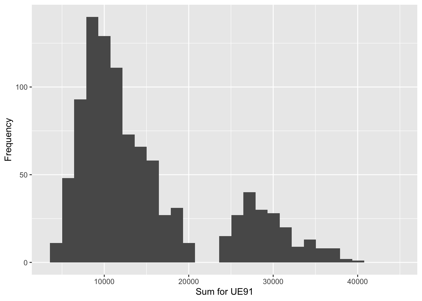
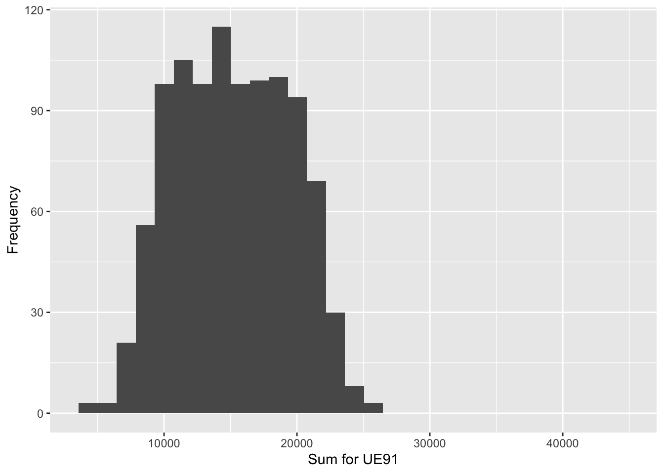
We use three different auxiliary variables in PPSWOR sampling. The first auxiliary variable is HOU85 (the number of households in the municipality). The two others are artificial variables x and z. These variables are constructed for pedagogical purposes to demonstrate the role of correlation of the study variable and auxiliary variable, and that a strong correlation alone does not guarantee good efficiency for PPSWOR. Further instructions are given once you start.

Start SAS Training Key

Simulation Experiments: the use of alternative auxiliary information in PPSWOR sampling

Select the desired size measure variable from the tab below and view the simulation results. Size variables that you can select are:

HOU85 (number of households in a municipality)
Z (artificially created variable for pedagogical purposes, N(500,150))
X (artificially created variable for pedagogical purposes, UE91 + 3000)

HOU85

**Simulation Experiments for PPS estimator for the total of UE91. Size variable HOU85, Sample size 8, Simulations 1000.**
Population_Total	Mean_of_Estimates	Std_error	Bias
15098	15118.36	455.1317	20.36347

Z

**Simulation Experiments for PPS estimator for the total of UE91. Size variable Z, Sample size 8, Simulations 1000.**
Population_Total	Mean_of_Estimates	Std_error	Bias
15098	14732.96	8192.497	365.0374

X

**Simulation Experiments for PPS estimator for the total of UE91. Size variable X, Sample size 8, Simulations 1000.**
Population_Total	Mean_of_Estimates	Std_error	Bias
15098	15175.88	4296.628	77.88458

C) INTERACTIVE SAS USE

Please download the SAS code for your own further training. Further instructions are given once you download the code.

NOTE! You need to have access to SAS in your computer.

Download SAS code

Chapter 2: Basic Sampling Techniques

2.2 The Province’91 population

TRAINING KEY 28: Analysing an SRS sample

INTRODUCTION

A) ANALYSING AN SRS SAMPLE FROM THE PROVINCE’91 POPULATION

B) SRS ESTIMATION WITH DIFFERENT SAMPLE SIZES

Different sample sizes (n=4,8,16 or 32) of SRSWOR sample

n=4

n=8

n=16

n=32

C) SIMULATING SRSWOR SAMPLES BY USING MONTE CARLO SIMULATION TECHNIQUES

Simulation Experiments for SRSWOR estimator for the total of UE91

n=4

n=8

n=16

n=24

TRAINING KEY 45: Intra-class correlation for systematic sampling

INTRODUCTION

A) INTRA-CLASS CORRELATION FOR SYSTEMATIC SAMPLING IN THE PROVINCE’91 POPULATION

B) INTRA-CLASS CORRELATION FOR SYSTEMATIC SAMPLING WHEN VARYING THE SORTING ORDER

C) INTERACTIVE SAS USE

TRAINING KEY 54: The use of auxiliary information in PPS sampling

INTRODUCTION

A) REFERENCE EXAMPLE 2.6: Estimation under systematic PPS sampling

B) THE USE OF ALTERNATIVE AUXILIARY INFORMATION IN PPSWOR SAMPLING

Simulation Experiments: the use of alternative auxiliary information in PPSWOR sampling

HOU85

Z

X

C) INTERACTIVE SAS USE

Further Reading

Chapter 2: Further Reading

TRAINING KEY 28: Analysing an SRS sample

TRAINING KEY 54: The use of auxiliary information in PPS sampling